Decision Tree Classifier from Scratch: Classifying Student’s Knowledge Level

Taking Small Steps Towards Data Science

Decision Tree Classifier from Scratch: Classifying Student’s Knowledge Level

Writing a Decision Tree Classifier from scratch using a python programming language

Prerequisites

You need to have basic knowledge in:

1. Python programming language
2. Numpy (Library for scientific computing)
3. Pandas

Data set

The data set I am going to use in this project has been sourced from the Machine Learning Repository of the University of California, Irvine User Knowledge Modeling Data Set (UC Irvine).
The UCI page mentions the following publication as the original source of the data set:

H. T. Kahraman, Sagiroglu, S., Colak, I., Developing intuitive knowledge classifier and modeling of users’ domain dependent data in web, Knowledge Based Systems, vol. 37, pp. 283–295, 2013

Introduction

1.1 What is a Decision Tree Classifier?

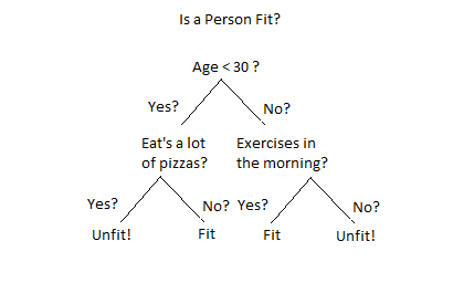
In simple words, a Decision Tree Classifier is a Supervised Machine learning algorithm that is used for supervised + classification problems. Under the hood in the decision tree, each node asks a True or False question about one of the features and moves left or right with respect to the decision.

You can learn more about Decision Tree from here.

1.2 What are we building?

We are going to use Machine Learning algorithms to find the patterns on the historical data of the students and classify their knowledge level, and for that, we are going to write our own simple Decision Tree Classifier from scratch by using Python Programming Language.

Though i am going to explain everything along the way, it will not be a basic level explanation. I will highlight the important concepts with further links so that everyone can explore more on that topic.

Code Part

2.1 Preparing Data

We are going to use pandas for data processing and data cleaning.

import pandas as pddf = pd.read_csv('data.csv')
df.head()

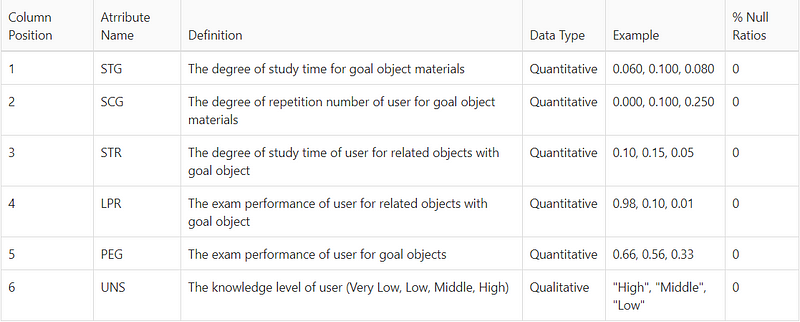
First off, we are importing the data.csv file then processing it as a panda’s data frame and taking a peek at the data.

As we can see our data has 6 columns. It contains 5 features and 1 label. Since this data is already cleaned, there is no need for data cleaning and wrangling. But while working with other real-world datasets it is important to check for null values and outliers in the dataset and engineer the best features out of it.

2.2 Train Test Splittrain = df.values[-:20]
test = df.values[-20:]

here we split our data into train and test where the last 20 data of our dataset are test data and the rest are train data.

2.3 Writing our own Machine Learning Model

Now it’s time to write our Decision Tree Classifier.

But before diving into code there are few things to learn:

1. To build the tree we are using a Decision Tree learning algorithm called CART. There are other learning algorithms like ID3, C4.5, C5.0, etc. You can learn more about them from here.
2. CART stands for Classification and Regression Trees. CART uses Gini impurity as its metric to quantify how much a question helps to unmix the data or in simple words CARD uses Gini as its cost function to evaluate the error.
3. Under the hood, all the learning algorithms give us a procedure to decide which question to ask and when.
4. To check how correctly the question helped us to unmix the data we use Information Gain. It helps us to reduce the uncertainty and we use this to select the best question to ask and given that question, we recursively build tree nodes. We then further continue dividing the node until there are no questions to ask and we denote that last node as a leaf.

2.3.1 Writing Helper functions

To implement the Decision Tree Classifier we need to know what question to ask about the data and when. Let's write a code for that:class CreateQuestion: def __init__(self, column, value):
self.column = column
self.value = value def check(self, data):
val = data[self.column]
return val >= self.value
def __repr__(self):

return "Is %s %s %s?" % (
self.column[-1], ">=", str(self.value))

Above we’ve written a CreateQuestion class that takes 2 inputs: column number and value as an instance variable. It has a check method which is used to compare the feature value.

__repr__ is just a python’s magic function to help display the question.

Let's see it in action:q = CreateQuestion(0, 0.08)

now let's check if our check method is working fine or not:data = train[0]
q.check(data)

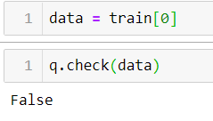
as we can see we’ve got a False value. Since our 0ᵗʰ value in the train set is 0.0 which is not greater than or equals to 0.08, our method is working fine.

Now it’s time to create a partition function that helps us to partition our data into two subsets: The first set contains all the data which is True and the second contains False.

Let's write a code for this:def partition(rows, qsn):

true_rows, false_rows = [], []
for row in rows:
if qsn.check(row):
true_rows.append(row)
else:
false_rows.append(row)
return true_rows, false_rows

our partition function takes two inputs: rows and a question then returns a list of true rows and false rows.

Let's see this in action as well:true_rows, false_rows = partition(train, CreateQuestion(0, 0.08))

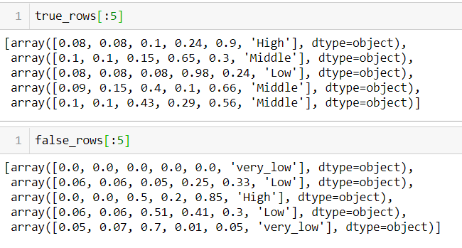
here true_rows contains all the data grater or equal to 0.08 and false_rows contains data less than 0.08.

Now it’s time to write our Gini Impurity algorithm. As we’ve discussed earlier, it helps us to quantify how much uncertainty there is in the node, and Information Gain lets us quantify how much a question reduces that uncertainty.

Impurity metrics range between 0 and 1 where a lower value indicates less uncertainty.

def gini(rows):counts = class_count(rows)
impurity = 1
for label in counts:
probab_of_label = counts[label] / float(len(rows))
impurity -= probab_of_label**2
return impurity

In our gini function, we have just implemented the formula for Gini. It returns the impurity value of given rows.

counts variable holds the dictionary with total counts of the given value in the dataset. class_counts is a helper function to count a total number of data present in a dataset of a certain class.def class_counts(rows):

for row in rows:

label = row[-1]
if label not in counts:
counts[label] = 0
counts[label] += 1
return counts

Let's see gini in action:

As you can see in image 1 there is some impurity so it returns 0.5 and in image 2 there are no impurities so it returns 0.

Now we are going to write code for calculating information gain:def info_gain(left, right, current_uncertainty):

p = float(len(left)) / (len(left) + len(right))
return current_uncertainty - p * gini(left) \
- (1 - p) * gini(right)

Information gain is calculated by subtracting the uncertainty starting node with a weighted impurity of two child nodes.

2.3.2 Putting it all together

Now it's time to put everything together.def find_best_split(rows):

best_gain = 0
best_question = None
current_uncertainty = gini(rows)
n_features = len(rows[0]) - 1

for col in range(n_features):

values = set([row[col] for row in rows])

for val in values:
question = Question(col, val)
true_rows, false_rows = partition(rows, question)if len(true_rows) == 0 or len(false_rows) == 0:
continue

gain = info_gain(true_rows, false_rows,\
current_uncertainty)if gain > best_gain:
best_gain, best_question = gain, question

return best_gain, best_question

We have written a find_best_split function which finds the best question by iterating over every feature and labels then calculates the information gain.

Let's see this function in action:best_gain, best_question = find_best_split(train)

We are now going to write our fit function.def fit(features, labels):data = features + labelsgain, question = find_best_split(data)

if gain == 0:
return Leaf(rows)

true_rows, false_rows = partition(rows, question)

# Recursively build the true branch.
true_branch = build_tree(true_rows)

# Recursively build the false branch.
false_branch = build_tree(false_rows)

return Decision_Node(question, true_branch, false_branch)

Our fit function basically builds a tree for us. It starts with the root node and finding the best question to ask for that node by using our find_best_split function. It iterates over each value then splits the data and information gain is calculated. Along the way, it keeps track of the question which produces the most gain.

After that, if there is still a useful question to ask, the gain will be grater then 0 so rows are sub-grouped into branches and it recursively builds the true branch first until there are no further questions to ask and gain is 0.

That node then becomes a Leaf node.

code for our Leaf class looks like this:class Leaf:

def __init__(self, rows):
self.predictions = class_counts(rows)

It holds a dictionary of class(“High”, “Low”) and a number of times it appears in the rows from the data that reached the current leaf.

for the false branch also the same process is applied. After that, it becomes a Decision_Node.

Code for our Decision_Node class looks like this:class Decision_Node:
def __init__(self, question,\
true_branch,false_branch):
self.question = question
self.true_branch = true_branch
self.false_branch = false_branch

This class just holds the reference of question we’ve asked and two child nodes that result.

now we return to the root node and build the false branch. Since there will not be any question to ask so, it becomes the Leaf node and the root node also becomes a Decision_Node.

Let's see fit function in action:_tree = fit(train)

to print the _tree we have to write a special function.def print_tree(node, spacing=""):

# Base case: we've reached a leaf
if isinstance(node, Leaf):
print (spacing + "Predict", node.predictions)
return

# Print the question at this node
print (spacing + str(node.question))

# Call this function recursively on the true branch
print (spacing + '--> True:')
print_tree(node.true_branch, spacing + " ")

# Call this function recursively on the false branch
print (spacing + '--> False:')
print_tree(node.false_branch, spacing + " ")

this print_tree function helps us to visualize our tree in an awesome way.

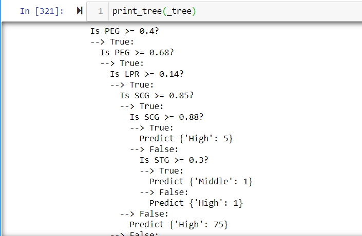
We have just finished building our Decision Tree Classifier!

To understand and see what we’ve built let's write some more helper functions:def classify(row, node):

if isinstance(node, Leaf):
return node.predictions

if node.question.check(row):
return classify(row, node.true_branch)
else:
return classify(row, node.false_branch)

classify function helps us to check the confidence by given row and a tree.classify(train[5], _tree)

as you can see above, our tree has classified the given value as a Middle with 96 confidence.def print_leaf(counts):

total = sum(counts.values()) * 1.0
probs = {}
for lbl in counts.keys():
probs[lbl] = str(int(counts[lbl] / total * 100)) + "%"
return probs

print_leaf function helps us to prettify our prediction.

2.4 Model Evaluation

We have successfully built, visualized, and saw our tree in action.

Now let's perform a simple model evaluation:for row in testing_data:
print ("Actual level: %s. Predicted level: %s" %
(df['LABEL'], print_leaf(classify(row, _tree))))

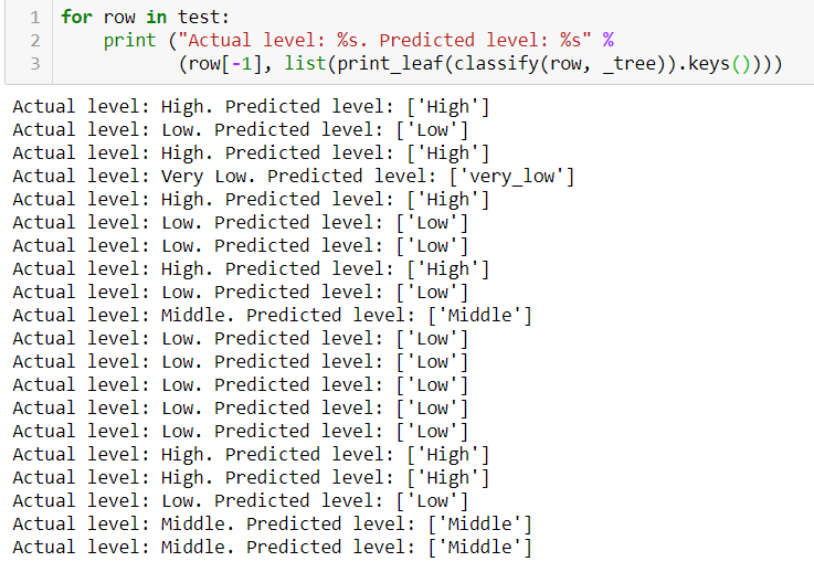
As you can see our tree nicely predicted our test data which was isolated from the train data.

Conclusion

Decision Tree Classifier is an awesome algorithm to learn. It is beginner-friendly and is easy to implement as well. We have built a very simple Decision Tree Classifier from scratch without using any abstract libraries to predict the student's knowledge level. By just swapping the dataset and tweaking few functions, you can use this algorithm for another classification purpose as well.

References

[1] H. T. Kahraman, Sagiroglu, S., Colak, I., Developing intuitive knowledge classifier and modeling of users’ domain-dependent data in web, Knowledge-Based Systems, vol. 37, pp. 283–295, 2013

[2] Aurelien Geron, Hands-on Machine Learning with Scikit-Learn, Keras & TensorFlow, O’REILLY, 2nd Edition, 2019