Core Learning Algorithm of Artificial Neural Network: Back-propagation Demystified

Opening the black box

Core Learning Algorithm of Artificial Neural Network: Back-propagation Demystified

Motivation

Recently at an ML interview, I was asked to explain how a back-propagation algorithm works.

I was not ready for that question and I didn’t know where to start. Though I had some understanding of how it works, it was all in my head. I could not figure out where to explain and what example to use.

So, the motivation behind this article is to demystify the back-propagation algorithm in possibly the simplest way so that ML beginners like us can explain it during the interviews and understand the underlying process of how this algorithm works.

Prerequisites

Before starting, I assume that you have some understanding of how artificial neural network works.

At least up to the point where you know what a typical neural network architecture looks like and what are the roles of input layers, hidden layers, synapses, weights, biases, output layers and cost functions. 😅

What is Back-propagation?

If you have started to learn about Machine Learning and Artificial Neural Networksa then you might have encountered the term Back-propagation.

Let’s look at the definition first and understand what it is and what it does:

Back-propagation, short for “backward propagation of errors,” is an algorithm for supervised learning of artificial neural networks using gradient descent. — Brilliant.org

Given an artificial neural network and an error function, the back-propagation algorithm calculates the negative gradient of the error function with respect to the weights of the network.

It is the core algorithm behind how an artificial neural network learns.

If it has been a while then you might have already understood the purpose of back-propagation.

In this article, rather than focusing on what it is, we are going to understand how it actually works and why it is so awesome.

Let’s try to understand it by the simplest example possible.

How it works? — As Simple As Possible

To understand the algorithm, let’s take an example of a simple artificial neural network with one input layer and one output layer.

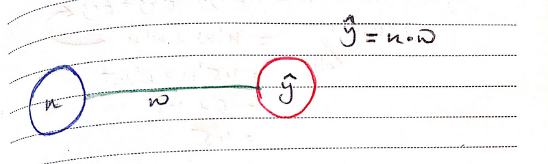
It has the input (x) with the weight (w) and an output (ŷ).

Note: Here we are not going to use any hidden layers, activation functions or add any bias unit.

Since we do not have any hidden layers and we are not using any activation function, our output (ŷ) is the multiplication of input (x) and weight (w):ŷ = x * w

Now, let’s say we have our training data with an input (x)=1.5The backpropagation and an expected output (y)=0.5.

+--———+--——————+
|input(x)   | expected output(y) |
+-----------+--------------------+
| 1.5       | 0.5                |
+--———+--——————+

By given input 1.5 we expect our network to produce the output 0.5.

let’s initialize our weight (w) with a random value w=0.8 and see what it produces.

1.5 * 0.8 = 1.2

+--———+--——————+—————+
|input(x)   | expected output(y) | output(ŷ)     |
+-----------+--------------------+---------------+
| 1.5       | 0.5                | 1.2           |
+--———+--——————+—————+

With the current weight, as you can see it produces 1.2.

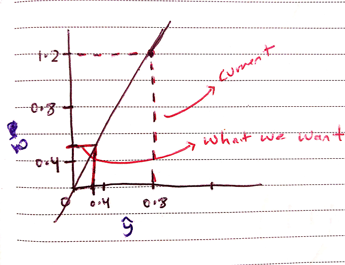
Now we need to define the error for our network through which it can learn how bad it performed.

For simplicity, let’s take the difference between the actual output and the expected output and then square it.j = (ŷ - y)²

Now that we have our error function (j), our job is to minimize it. The backpropagation algorithm seeks to do it by descending along the error function: this is called Gradient Descent.

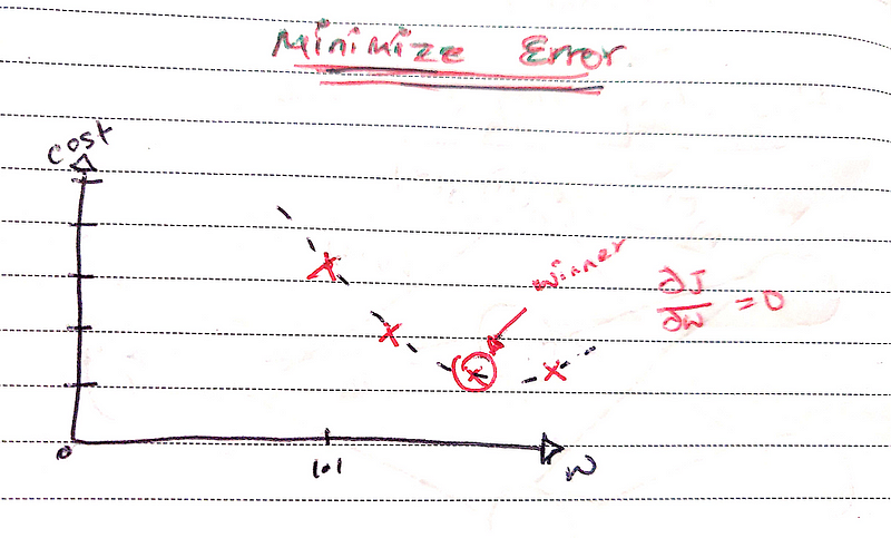
Gradient Descent deserves a separate explanation, but in simple words: It looks at the slope of the tangent line at a given point of the error function and figures out which way is downhill.

Now in order to perform the back-propagation, we need to calculate the derivative(rate of change) of our error function (j).

Since we do not have much control over our network, we will minimize our error by changing the weight (w).

Our expression for the rate of change in (j) with respect to (w) will be:

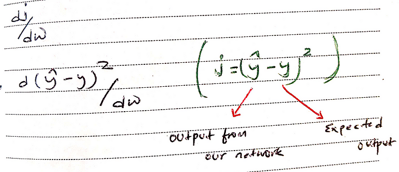
To calculate our first derivative we have to use the chain rule of differentiation.

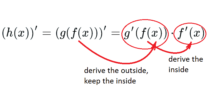
The chain rule tells us how to take the derivative of a function inside the function and the power rule tells us to bring down our exponent 2 and multiply it.

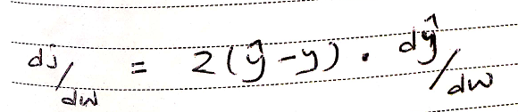
Note: Here we are taking the derivative of our outside function and multiplying with our inside function. Since y=0.5 which is a constant, derivative of constant is 0 and also it does not change with respect to w so we are left with dŷ/dw.dj/dw = 2(ŷ - y)*d(ŷ)/dw

Since ŷ=x.w: dj/dw = 2(ŷ - y) *d(1.5 * w)/d(w) = 2(ŷ-y)*1.5 = 4.5w - 1.5

now that we have our equation : dj/dw = 4.5w-1.5 let’s perform Gradient Descent.

We are basically going to deduct the rate of change in our error function with respect to weight from our old weight and along the way, we are going to multiply the change with our learning rate (lr) = 0.1.

Note: Learning rate defines how big step we want to take.

Our formula to descent our gradient will be:w(new) := w(old)-lr(dj/dw)
w(new) := w(old) - 0.1(4.5w(old) - 1.5)

Now let’s calculate our new weight with that formula:

+--———+--——————+
|old weight | new weight         |
+-----------+--------------------+
| 0.8       | 0.59               |
+-----------+--------------------+
| 0.59      | 0.4745             |
+-----------+--------------------+
| 0.4745    | 0.410975           |
+-----------+--------------------+
| 0.410975  | 0.37603625         |
+-----------+--------------------+
| 0.37603625| 0.3568199375       |
+-----------+--------------------+
+------------+-----------+
|0.3568199375| 0.333333  |
+————+--———+

We have successfully trained our neural network.

The optimal weight for our network is 0.333.

1.5 * 0.333 = 0.5

+--———+--——————+—————+
|input(x)   | expected output(y) | output(ŷ)     |
+-----------+--------------------+---------------+
| 1.5       | 0.5                | 0.5           |
+--———+--——————+—————+

Final Words

This is how the underlying process of back-propagation works to find out the optimal weights on artificial neural networks.

We have seen the process for a very simple network without any activation function or biases. However, in the real world also the process is the same but a bit complex since we have to propagate backward to many hidden layers with non-linearity and bias units.

For the interviews and to express your understanding, this much explanation is sufficient i suppose.

Not your cup of tea?

If this explanation also does not click your brain or you want to learn more then you can follow Neural Network tutorial series by 3Blue1Brown and Neural Network Demystified series by Welch Labs.

They have also explained the step-by-step process with nice visual representations.

Or if you want to learn it from a different perspective then here is a nice explanation from Brandon.

Hope you have learned something 😀. Thanks for reading.