
Fake News Classification using GLOVE and Long Short Term Memory (LSTM)

Fake News Classification using Long Short Term Memory (LSTM)
Using a deep learning model to classify whether the news is fake or not from the election news article data set
Introduction
In this tutorial, we are going to develop a Fake News Classifier using Long Short Term Memory (LSTM).
We are going to write our LSTM model using Python programming Language and Keras deep learning library on Spell Platform’s Workspace.
Prerequisites
Before getting started, you should have a good understanding of:
- Python programming language
- Keras — Deep learning library
Dataset
For our project, we are going to use fake_or_real_news.csv dataset which I found on GitHub. There are many other open source datasets available; you can use any other of your choice. Some of the options are:
- Liar Dataset — URL: https://www.cs.ucsb.edu/~william/data/liar_dataset.zip
- Fake News Corpus — URL: https://github.com/several27/FakeNewsCorpus
- Fake News Detection Resources — URL: https://github.com/mdepak/fake-news-detection-resources
The dataset we are using is the news articles written around the 2016 US election period.
Preparations
Getting Our Workspace Ready
To get started, let’s login to the Spell platform and head to the Workspaces tab.
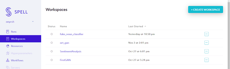
Note: If you are using Spell for the first time then you should see a blank workspace and a “Create Workspace” button.
You can create your new workspace using the Create Workspace button.
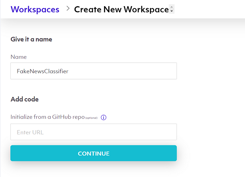
Give your workspace any name and hit continue.
After that, you have an option to select your machine type and install the required libraries for the project.
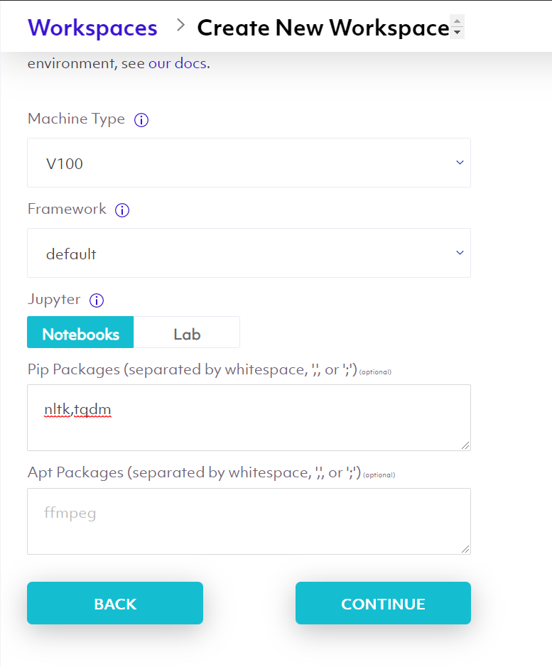
For this project we are using a V100 machine type and a Jupyter Notebook.
All the common libraries are pre-installed in Spell, but for our project we require some extra libraries so we are mentioning them in the Pip Packages section.
We are using NLTK for removing stopwords from our dataset and tqdm for just a nice progress bar on our notebook.
After that, we hit continue.
Now we have to mount our dataset folder, but before that, we have to upload our data on Spell.
Let’s do that first.
Getting The Dataset Ready
In our command line, let’s enter the following command:pip install spell
This command will install Spell CLI on our local machine.
After that:spell login
This will ask us for our Spell credentials; just enter the credentials and we are good to go.
After a successful login, we can now upload our dataset file.
We’ve downloaded the fake_or_real_news.csv on our local machine, so let’s upload that on Spell.
To do that, let’s head to our project folder, open a command prompt and enter the following command:spell upload fake_or_real_news.csv
This will upload our dataset file on our desired directory on Spell.
Getting Glove Vector Ready
In this project, we are going to use pre-trained Glove Vectors for word embeddings. We will be getting back to Glove Vectors later on in this tutorial; for now, we can just download the file from their official site: https://nlp.stanford.edu/projects/glove/
For this project, we are using glove6B file which contains vector representations of Wikipedia 2014 and Gigaword 5. It has 6 billion tokens, 400 thousand vocab, and 50, 100, 200 dimension, & 300 dimensional vectors which is of 822 MB size.
For this project we are going to use the 100d vector file, let’s upload that on Spell as well.spell upload glove.6B.100d.txt
Note: while uploading, Spell will ask you to choose your directory name; upload your data file to your desired directory.
Getting Jupyter Notebook Ready
Now that we have uploaded everything we need on Spell, let’s mount the dataset and glove directories on our workspace and complete the creation process.
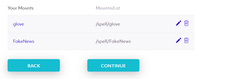
Here, we have glove files in the glove directory and our dataset in the FakeNews directory.
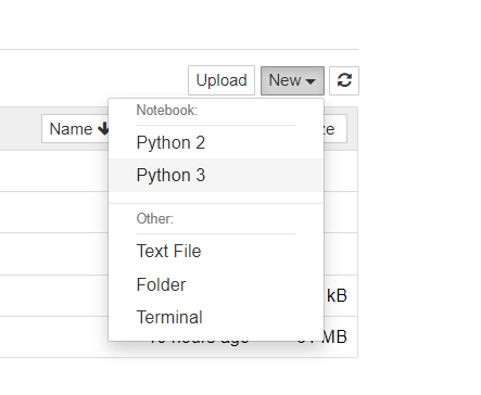
Now, after pressing the continue button, we can see our GPU powered Jupyter Notebook workspace with our dataset folders.

Let’s create our notebook file and start writing our code.
Importing all the required libraries
Before getting started with our code, let’s import all the required libraries:import re
from tqdm import tqdm_notebook
from nltk.corpus import stopwordsfrom tensorflow.keras import regularizers, initializers, optimizers, callbacks
from tensorflow.keras.preprocessing.sequence import pad_sequences
from tensorflow.keras.preprocessing.text import Tokenizer
from keras.utils.np_utils import to_categorical
from tensorflow.keras.layers import *
from tensorflow.keras.models import Sequential
import pandas as pd
import numpy as np
Here we are importing essential libraries for developing our Keras model from tensorflow.keras and we are using nltk’s stopwords method to remove stopwords from our data, numpy for array operations and pandas to process data.
Load and Process Data
The next step is to load our dataset files and structure them into a format that we can work with.
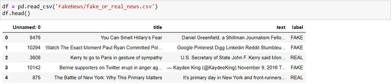
Let’s load our data file Fake_or_real_news.csv using pandas.df = pd.read_csv(‘FakeNews/fake_or_real_news.csv’)
df.head()
Out:
Let’s see the info of our dataset:df.info()
Out:
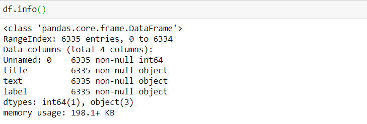
We have a total of 6335 entries and no null values.
From our dataset we need title, text and label. Let’s extract them out.x = df[‘title’] + “ “ + df[‘text’]
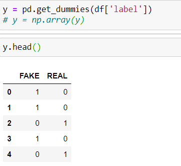
y = pd.get_dummies(df[‘label’])
y = np.array(y)
Here we are concatenating the title and the text row and storing them on x variable and on y variable we are re-storing a one-hot vector of our label data.
Let’s see how our features and labels look:
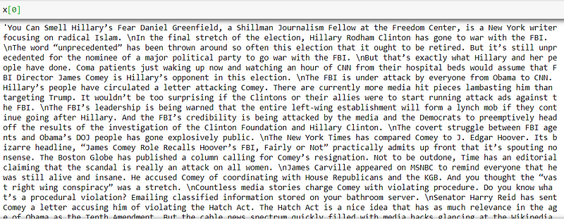
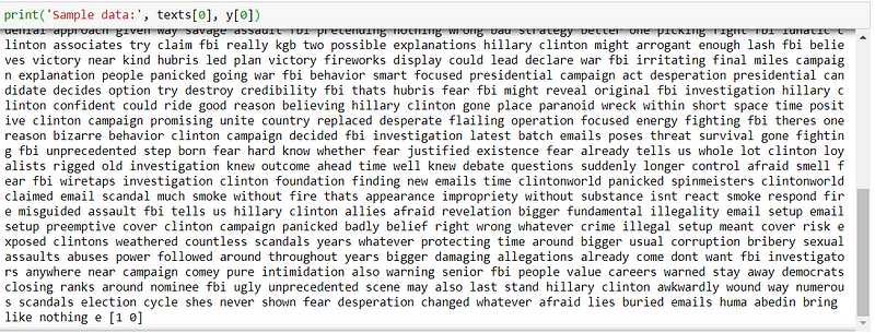
As we can see our x variable has a bunch of text which is the concatenation of title and text values.
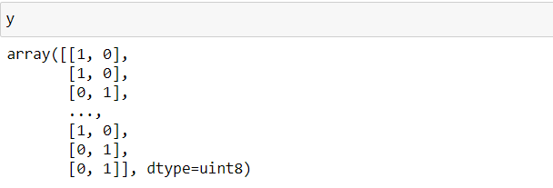
And on our y variable we have one-hot vectors of our Fake or Real values.
Pandas get_dummies() function will convert our column into n number of different columns with respect to the unique values in our column and later we are just converting those pandas series to numpy array.
Defining Parameters
Let’s define some parameters for our Model.MAX_NB_WORDS = 100000 # max number of words for tokenizer
MAX_SEQUENCE_LENGTH = 1000 # max length of each sentences, including padding
VALIDATION_SPLIT = 0.2 # 20% of data for validation (not used in training)
EMBEDDING_DIM = 100 # embedding dimensions for word vectors
GLOVE_DIR = “glove/glove.6B.”+str(EMBEDDING_DIM)+”d.txt”
“MAX_NB_WORDS” defines the max number of words for tokenizer.
“MAX_SEQUENCE_LENGTH” defines the max length for our corpus. If any rows of our data does not match this length we are going to add padding on it.
“VALIDATION_SPLIT” defines how much data we want to separate from our dataset for validation purpose. Those data are not included in the training process.
“EMBEDDING_DIM” defines the embedding dimensions for our Glove vectors.
“GLOVE_DIR” defines the path to our glove vectors.
Data Cleaning
In our dataset we have to look for any stopwords or unnecessary characters and remove them for our model to perform better.
Stopwords are the commonly used words such as “the”, “a”, “an”, “in”. They do not mean anything to our model so we are filtering them.
Let’s write a function for data cleaning:def clean_text(text, remove_stopwords = True):
output = “”
text = str(text).replace(r’http[\w:/\.]+’,’’) # removing urls
text = str(text).replace(r’[^\.\w\s]’,’’) #remove everything but characters and punctuationtext = str(text).replace(r’\.\.+’,’.’) #replace multiple periods with a single onetext = str(text).replace(r’\.’,’ . ‘) #replace periods with a single onetext = str(text).replace(r’\s\s+’,’ ‘) #replace multiple white space with a single onetext = str(text).replace(“\n”, “”) #removing line breaks
text = re.sub(r’[^\w\s]’,’’,text).lower() #lower textsif remove_stopwords:
text = text.split(“ “)
for word in text:
if word not in stopwords.words(“english”):
output = output + “ “ + word
else:
output = text
return str(output.strip())[1:-3].replace(“ “, “ “)
Let’s break it down:
In our clean_text function we are removing unnecessary characters and data like URLs, line breaks, double whitespaces and stopwords and making everything lowercase, then returning the cleaned data on the output variable.
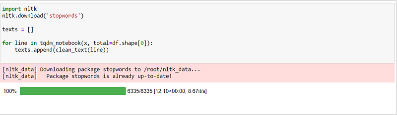
For our remove_stopwords to work, we have to first download the stopwords package from nltk.import nltk
nltk.download(‘stopwords’)
After downloading the stopwords, let’s see our clean_text function in action:texts = []for line in tqdm_notebook(x, total=df.shape[0]):
texts.append(clean_text(line))
Here we are iterating over each row of our dataset and cleaning them, then appending them on our texts list.
We are using tqdm for a nice progress bar on our notebook.
Now let's see our data and label:print(‘Sample data:’, texts[0], y[0])
Out:
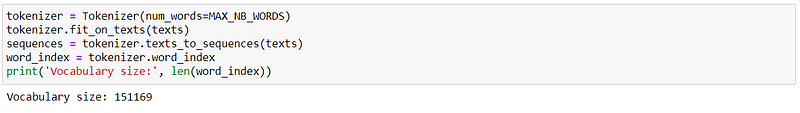
Tokenization
The next step is to tokenize our data. We are using Keras Tokenizer. After that, we are building a word_index from it.tokenizer = Tokenizer(num_words=MAX_NB_WORDS)
tokenizer.fit_on_texts(texts)
sequences = tokenizer.texts_to_sequences(texts)
word_index = tokenizer.word_index
print(‘Vocabulary size:’, len(word_index))
Out:
Padding
Now we are going to add padding to our data to make it uniform. Keras makes it easy to pad our data by using pad_sequences function.data = pad_sequences(sequences, padding = ‘post’, maxlen = MAX_SEQUENCE_LENGTH)
print(‘Shape of data tensor:’, data.shape)
print(‘Shape of label tensor:’, y.shape)
Out:
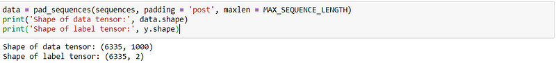
As we can see, we have 6335 total data with a length of 1000 which is the MAX_SEQUENCE_LENGTH for our features.
And for our labels, we have total 6335 data and length 2.
Shuffling
Now we are just randomly shuffling our data.indices = np.arange(data.shape[0])
np.random.shuffle(indices)
data = data[indices]
labels = y[indices]
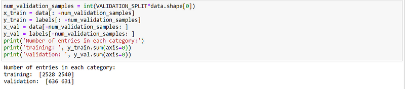
Split
The next step is to split our data into training and validation sets. We are splitting our data into 20% for validation and the rest for training.num_validation_samples = int(VALIDATION_SPLIT*data.shape[0])
x_train = data[: -num_validation_samples]
y_train = labels[: -num_validation_samples]
x_val = data[-num_validation_samples: ]
y_val = labels[-num_validation_samples: ]
print(‘Number of entries in each category:’)
print(‘training: ‘, y_train.sum(axis=0))
print(‘validation: ‘, y_val.sum(axis=0))
Out:
Let’s look at our tokenized data:print(‘Tokenized sentences: \n’, data[10])
print(‘One hot label: \n’, labels[10])OUT:
Tokenized sentences:
[ 8965 231 18835 5813 1003 12678 2268 39260 38336 1042 5452 543
8570 16443 5013 29202 39261 407 4820 91082 154 6836 1078 12550
5568 30936 91083 53 29202 159 16575 1139 5074 465 1478 90
166 72 407 5453 4820 154 6836 1114 13853 420 91084 2815
163 19 21062 2355 133 12900 5624 6216 3218 962 148 22530
14950 32858 1317 7902 521 3667 29202 242 78 39262 5074 2815
237 4674 91085 1732 28950 3830 13034 12040 91086 877 1968 19523
6344 19330 91087 836 21547 16072 39263 674 858 91088 21360 566
362 6781 2815 1317 3264 11802 50578 2036 10934 561 7195 2503
18390 583 1367 1476 50578 3830 1760 91089 337 765 625 63
261 561 9405 288 13 1317 281 10934 6781 2815 638 26
625 63 60 489 66 170 278 79 172 199 2974 923
1953 278 253 5939 2268 159 672 1011 2669 522 2921 2268
7697 2761 82 21799 50579 23 576 63 199 121 2503 328
6605 170 278 79 3934 199 5852 939 4 2268 91090 63
198 13 1317 15 2935 715 383 5358 1078 10735 7353 8
1108 66 5481 91091 7353 1078 12550 3945 5584 638 26 72
91092 117 22 50036 765 408 26 72 11 1262 101 79
63 71 22914 10766 170 278 3818 6781 2815 2237 11696 4
4239 7280 91093 19 5013 29202 6615 6781 2815 765 1387 231
391 91094 154 663 753 63 765 79 770 6781 11696 15
121 91095 422 4978 3149 5074 422 32858 5 414 128 349
283 128 8628 322 1041 2394 6362 134 13401 25014 2477 170
278 79 414 128 15 50580 5939 961 2477 4631 765 9973
1360 15 5520 79 9 305 63 1713 93 888 26 202
191 172 482 50581 3744 6781 3220 28237 21165 265 132 388
32 221 21722 414 128 5301 248 32 542 3928 289 677
6171 26325 20034 733 5580 289 677 146 26326 27971 626 305
289 677 327 609 6455 2959 74 243 16 584 15538 13038
13157 6 3322 983 6773 3998 724 743 278 1124 11186 9
442 16 2305 53 219 91096 700 289 677 2066 1222 13737
9 11903 4770 298 6271 298 5454 2852 15 103 1396 170
50582 13681 2314 177 221 27 8397 1206 365 101 1682 18203
279 345 1689 11621 19047 32 21 627 5622 12268 20009 8069
25020 12652 265 132 26 272 261 765 4498 257 5524 237
25916 348 63 90 151 765 4498 101 1682 87 10295 90
21101 112 257 15 44702 3214 846 6455 1665 1420 1052 2046
1588 10 119 68 15651 84 12966 15 10169 1554 1320 414
128 961 1238 21 10332 101 1819 2477 170 278 26 1255
18 182 4 136 971 5708 13038 50583 168 24637 8736 2314
6195 379 15 29203 23 4933 8277 1575 91097 27 101 1682
16473 6152 7 778 9242 939 32 63 931 30 27 153
88 1530 8744 601 4 69 339 752 436 21076 91098 15141
3852 5440 2237 91099 4256 6781 91100 278 622 384 318 107
38 1326 32 1855 789 3935 18 182 334 6830 680 15118
5939 13959 32 1402 11 18 1184 12941 17147 8143 9464 50584
79 147 3455 117 1810 83 105 128 10542 32 10023 182
11353 5708 2797 1823 5545 601 74 5059 5708 2797 163 13
182 8572 813 2797 147 625 393 3052 32 77 79 5347
130 117 90 10395 480 6722 79 32 17285 91101 91102 11
2531 8792 79 4124 7864 1 32 652 146 940 5985 300
11 3491 1020 824 18579 2472 2173 711 198 87 734 33020
21 221 3535 3782 18 7042 945 693 1294 10382 41 2318
7042 1441 765 174 825 3354 317 1379 63 337 14185 79
1444 1803 71 174 15184 6781 91103 7643 257 5025 1041 2394
6362 28149 134 660 42 24194 74 83 761 13170 1218 625
63 5440 2237 10766 4256 33231 170 278 91104 814 27 24992
91105 5013 29202 2036 2276 1326 241 8570 6781 1592 1506 2237
1003 7 6615 170 91106 4034 3168 2911 1165 221 284 39
1554 1320 434 1957 66 828 5654 117 1200 3917 84 215
2635 6807 20076 0 0 0 0 0 0 0 0 0
0 0 0 0 0 0 0 0 0 0 0 0
0 0 0 0 0 0 0 0 0 0 0 0
0 0 0 0 0 0 0 0 0 0 0 0
0 0 0 0 0 0 0 0 0 0 0 0
0 0 0 0 0 0 0 0 0 0 0 0
0 0 0 0 0 0 0 0 0 0 0 0
0 0 0 0 0 0 0 0 0 0 0 0
0 0 0 0 0 0 0 0 0 0 0 0
0 0 0 0 0 0 0 0 0 0 0 0
0 0 0 0 0 0 0 0 0 0 0 0
0 0 0 0 0 0 0 0 0 0 0 0
0 0 0 0 0 0 0 0 0 0 0 0
0 0 0 0 0 0 0 0 0 0 0 0
0 0 0 0 0 0 0 0 0 0 0 0
0 0 0 0 0 0 0 0 0 0 0 0
0 0 0 0 0 0 0 0 0 0 0 0
0 0 0 0 0 0 0 0 0 0 0 0
0 0 0 0 0 0 0 0 0 0 0 0
0 0 0 0 0 0 0 0 0 0 0 0
0 0 0 0 0 0 0 0 0 0 0 0
0 0 0 0 0 0 0 0 0 0 0 0
0 0 0 0 0 0 0 0 0 0 0 0
0 0 0 0]
One hot label:
[0 1]
This is a tokenized vector representation of our data at 10th index. The 0 values at the end are the padding to make our data length uniform.
Word Embedding
Now we are going to implement word embeddings.
Before implementation, let’s understand what word embedding and Glove vectors are.
Word Embeddings
Word embedding algorithms can figure out tons of relationships from the text data. They use the idea of context and learn by seeing what word occurs near other words.
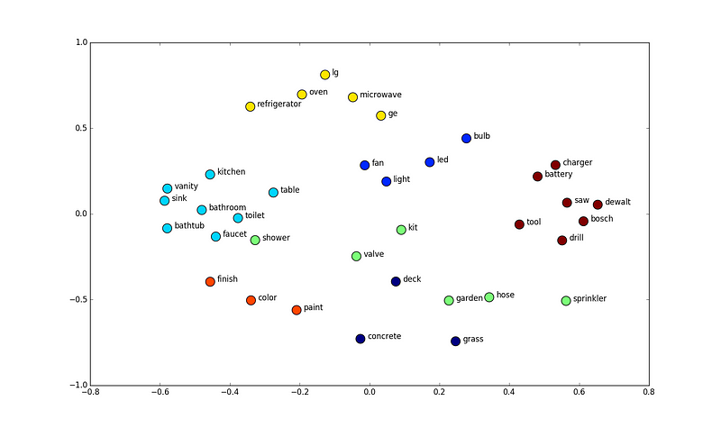
The picture above is the vector space of word embeddings. There we can see the closely related words are clustered together. For example: we have a kitchen, table, sink, bathroom, bathtub clustered together because they are closely related. And also we have a charger, battery, saw, drill, tool, etc. clustered together because they represent tools.
You can see a cool example of word embedding here:https://embeddings.macheads101.com/
In this demo app developed by macheads101, if we enter a food name then it will give us a bunch of other food names by understanding the context. Cool right?
There are many popular word embedding algorithms available out there. Glove and Word2Vec are the most popular ones.
For our project we are going to use pre-trained weights of Glove vector which is available on their official site to download.
Glove Vectors
As we have already downloaded Glove vectors pre-trained weights earlier and uploaded them on Spell, let’s understand Glove first.
Glove is an unsupervised learning algorithm for obtaining vector representations for words. Training is performed on aggregated global word-word co-occurrence statistics from a corpus, and the resulting representations showcase interesting linear substructures of the word vector space.
If we have sufficient corpus data then we can train our own glove vector, but for this project we are using pre-trained 100 dimension glove vector.
What is 100d? Why 100d?
These dimensions are often selected in a fairly experimental way. It has nothing to do with our corpus or vocab size. I have randomly selected 100d and it performed fine so I’ve chosen to go with 100d.
Smaller dimension will represent the information contained in the corpus more compactly and will make it easier for the algorithm to leverage that information. In contrast, larger dimensions will capture more information but are harder to use.
Let’s write the code to represent our data on embedding index.embeddings_index = {}
f = open(GLOVE_DIR, encoding=’utf8')
print(‘Loading Glove from:’, GLOVE_DIR,’…’, end=’’)
for line in f:
values = line.split()
word = values[0]
embeddings_index[word] = np.asarray(values[1:], dtype=’float32')
f.close()
print(“Done.\n Proceeding with Embedding Matrix…”, end=””)embedding_matrix = np.random.random((len(word_index) + 1, EMBEDDING_DIM))
for word, i in word_index.items():
embedding_vector = embeddings_index.get(word)
if embedding_vector is not None:
embedding_matrix[i] = embedding_vector
print(“Completed!”)
This block of code will open our glove vector file and map words from our dataset to known embedding by parsing the data dump of pre-trained embedding.
Model
We have finished data preprocessing and word embedding. Now our next step is to create a model. We are going to create a sequential model, with Embedding and LSTM layer.
Long Short Term Memory (LSTM)
LSTM is a variant of Recurrent Neural Network (RNN) which has a memory cell. It performs better than vanilla RNN on long sequential data. LSTM was designed to overcome the vanishing gradient problem in RNN.
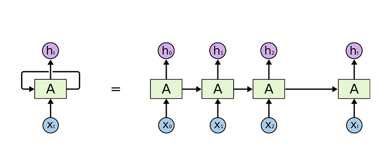
This is a vanilla recurrent neural network. They are basically designed in such a way that they can deal with sequential data. RNN’s recurrently take the input and output of the previous node.
Unlike feed forward neural networks, RNNs can use their internal state (memory) to process sequences of inputs. RNN uses the Back propagation Through Time (BPTT) algorithm to update weights, because when dealing with large sequence data, gradient starts vanishing. So to overcome that problem, LSTM was introduced.
In LSTM all the vanilla cells of RNN are replaced with a LSTM cell.
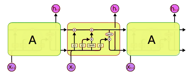
LSTM cells are composed of several gates like input, output and forget gates to preserve memory to a certain extent. At each timestep, LSTM cell can choose to read, write or reset the cell by using an explicit gating mechanism.
There is a lot of math involved in LSTM — to know more about the underlying process of how LSTM works you can read this nice post.
Model Initialization
Let’s create our sequential model and add layers:model = Sequential()
model.add(Input(shape=(MAX_SEQUENCE_LENGTH,), dtype=’int32'))
model.add(Embedding(len(word_index) + 1,
EMBEDDING_DIM,
weights = [embedding_matrix],
input_length = MAX_SEQUENCE_LENGTH,
trainable=False,
name = ‘embeddings’))
model.add(LSTM(60, return_sequences=True,name=’lstm_layer’))
model.add(GlobalMaxPool1D())
model.add(Dropout(0.1))
model.add(Dense(50, activation=”relu”))
model.add(Dropout(0.1))
model.add(Dense(2, activation=”sigmoid”))
Our first layer will be an input layer which takes the max sequence length of our data (1000).
Our second layer will be an Embedding layer. We feed our embedding matrix which we’ve created earlier to the embedding layer and set trainable to false. This is because we are using the pre-trained weights vector and we don’t want to train it again.
After creating our embedding sequences, it’s time to define the LSTM layer which returns the sequence data. We are also using a GlobalMaxPool layer of 1 dimension and dropouts. Our final layer is a dense layer which is of length 2 because our labels are one-hot vectors of length 2.
Model and hyperparameters has been sourced from this post of Susan Li
Train Model
Now that we have created our model, let’s compile and train them.model.compile(optimizer=’adam’, loss=’binary_crossentropy’,
metrics = [‘accuracy’])
We are using adam as our optimizer and binary_crossentropy as our loss function.
Let’s train our model:history = model.fit(x_train, y_train, epochs = 10, batch_size=128, validation_data=(x_val, y_val))
Here we are only using 10 epochs because using more epochs resulted in overfitting. And we are using batch size of 128 because in testing, 128 size worked fine. You are free to tweak the hyper parameters and test at your own.Train on 5068 samples, validate on 1267 samples
Epoch 1/10
5068/5068 [==============================] — 81s 16ms/sample — loss: 0.6540 — acc: 0.6124 — val_loss: 0.5471 — val_acc: 0.7482
Epoch 2/10
5068/5068 [==============================] — 80s 16ms/sample — loss: 0.4601 — acc: 0.7927 — val_loss: 0.3780 — val_acc: 0.8425
Epoch 3/10
5068/5068 [==============================] — 80s 16ms/sample — loss: 0.3565 — acc: 0.8513 — val_loss: 0.3357 — val_acc: 0.8520
Epoch 4/10
5068/5068 [==============================] — 79s 16ms/sample — loss: 0.3030 — acc: 0.8713 — val_loss: 0.2999 — val_acc: 0.8725
Epoch 5/10
5068/5068 [==============================] — 80s 16ms/sample — loss: 0.2805 — acc: 0.8818 — val_loss: 0.2756 — val_acc: 0.8895
Epoch 6/10
5068/5068 [==============================] — 80s 16ms/sample — loss: 0.2549 — acc: 0.8898 — val_loss: 0.3189 — val_acc: 0.8654
Epoch 7/10
5068/5068 [==============================] — 80s 16ms/sample — loss: 0.2504 — acc: 0.8933 — val_loss: 0.2502 — val_acc: 0.8990
Epoch 8/10
5068/5068 [==============================] — 79s 16ms/sample — loss: 0.2041 — acc: 0.9168 — val_loss: 0.2444 — val_acc: 0.9069
Epoch 9/10
5068/5068 [==============================] — 78s 15ms/sample — loss: 0.1850 — acc: 0.9240 — val_loss: 0.2317 — val_acc: 0.9116
Epoch 10/10
5068/5068 [==============================] — 79s 16ms/sample — loss: 0.1675 — acc: 0.9340 — val_loss: 0.2246 — val_acc: 0.9179
Our model did well, we have a validation accuracy of 91% which is a nice score.
Evaluate Model
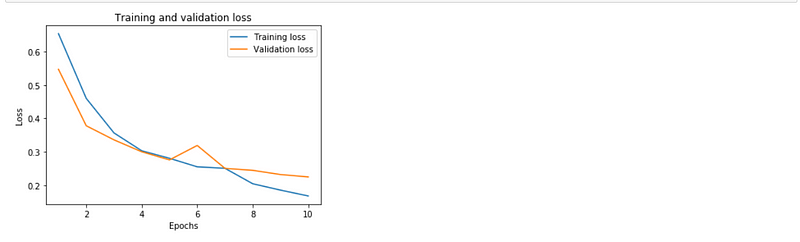
Now that we have trained our model, let’s look visually at how it did.
We are going to use matplotlib to visualize our train and validation’s accuracy and loss as well.import matplotlib.pyplot as plt%matplotlib inlineloss = history.history[‘loss’]
val_loss = history.history[‘val_loss’]
epochs = range(1, len(loss)+1)
plt.plot(epochs, loss, label=’Training loss’)
plt.plot(epochs, val_loss, label=’Validation loss’)
plt.title(‘Training and validation loss’)
plt.xlabel(‘Epochs’)
plt.ylabel(‘Loss’)
plt.legend()
plt.show();
accuracy = history.history[‘acc’]
val_accuracy = history.history[‘val_acc’]
plt.plot(epochs, accuracy, label=’Training accuracy’)
plt.plot(epochs, val_accuracy, label=’Validation accuracy’)
plt.title(‘Training and validation accuracy’)
plt.ylabel(‘Accuracy’)
plt.xlabel(‘Epochs’)
plt.legend()
plt.show();
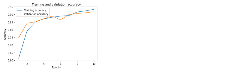
As we can see both our train and validation scores are good. Now let’s test our model with some random data from our dataset.random_num = np.random.randint(0, 100)
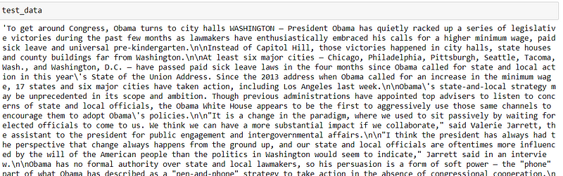
test_data = x[random_num]
test_label = y[random_num]clean_test_data = clean_text(test_data)
test_tokenizer = Tokenizer(num_words=MAX_NB_WORDS)
test_tokenizer.fit_on_texts(clean_test_data)
test_sequences = tokenizer.texts_to_sequences(clean_test_data)
word_index = test_tokenizer.word_index
test_data_padded = pad_sequences(test_sequences, padding = ‘post’, maxlen = MAX_SEQUENCE_LENGTH)
Here we are just picking random data from our dataset and processing them.
After that we are feeding that data into our model.prediction = model.predict(test_data_padded)
Let’s check our predictions:prediction[random_num].argsort()[-len(prediction[random_num]):]
Out:
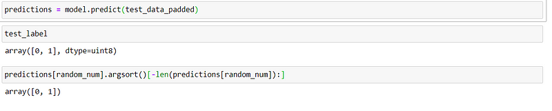
As we can see our model predicted correctly.
Test data preview:
Conclusion
We’ve trained our simple LSTM model on a fake news dataset and got an accuracy of 91%. There are many other machine learning models which perform much better but let’s admit it Machine Learning models require a lot of feature engineering and data wrangling. We are using a deep learning model to let the model figure everything out on its own.
You can further increase model size, tweak the hyperparameters, use Bidirectional LSTM and test if the model performs better. Also you can prepare a web API for this model, deploy it somewhere and create an application on top of it.
For any queries and discussion, you can join the Spell community from here: https://chat.spell.ml/
References
[1] Glove: Global Vectors of Word Representation, Jeffery Pennington, 2014
[2] Keras.io: Train an LSTM model, keras, [Online] https://keras.io/examples/imdb_lstm/
[3] Understanding LSTM Networks, colah, 2015,
[Online] https://colah.github.io/posts/2015-08-Understanding-LSTMs/

Comments ()