Generating Modern Art using Generative Adversarial Network(GAN)

Prerequisites

You need to have a good understanding of:

1. Image processing
2. Python Programming Language
3. Numpy — Scientific Computing Library
4. Keras — Deep Learning Library

And some basic knowledge of:

1. Generative Adversarial Network (GAN)

Dataset Used

Image data used in this project has been collected from WikiArts.org.

Introduction

In this tutorial, we are going to look at the step by step process to create a Generative Adversarial Network to generate Modern Art and write a code for that using Python and Keras together.

After that, for training the model, we are going to use a powerful GPU Instance of Spell platform. Everything will be explained along the way and links will be provided for further readings.

Let’s get started!

Exploring Dataset

Before getting started, let’s look at our image dataset.

WikiArt has a huge collection of modern art with various different styles. For our particular project, we are going to use images of Cubism Style.

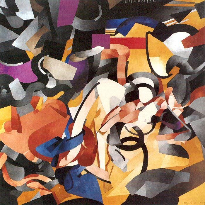
You can know more about the art styles and Modern Art from WikiArt.org.

Downloading Images

You can either download images that you like from WikiArt or head to this repository by cs-chan to download the 26GB of WikiArt images.

Since it has a collection of all the different types, we are only going to pick cubism and store them in folder named dataset.

Processing Image Data

Images in our dataset are of different sizes, to feed them into our Generative Adversarial Neural Network we are going to resize all our images to 128X128.

Before starting, create a python file at the root directory where your dataset folder is located.

Now let’s write a small python script to select all the images from the folder and resize them to 128X128 and save them on cubism_data.npy file.

## image_resizer.py
# Importing required libraries
import os
import numpy as np
from PIL import Image

# Defining an image size and image channel
# We are going to resize all our images to 128X128 size and since our images are colored images
# We are setting our image channels to 3 (RGB)

IMAGE_SIZE = 128
IMAGE_CHANNELS = 3
IMAGE_DIR = 'dataset/'

# Defining image dir path. Change this if you have different directory
images_path = IMAGE_DIR 

training_data = []

# Iterating over the images inside the directory and resizing them using
# Pillow's resize method.
print('resizing...')

for filename in os.listdir(images_path):
    path = os.path.join(images_path, filename)
    image = Image.open(path).resize((IMAGE_SIZE, IMAGE_SIZE), Image.ANTIALIAS)

    training_data.append(np.asarray(image))

training_data = np.reshape(
    training_data, (-1, IMAGE_SIZE, IMAGE_SIZE, IMAGE_CHANNELS))
training_data = training_data / 127.5 - 1

print('saving file...')
np.save('cubism_data.npy', training_data)

Let’s break it down.

In our code block above, in the first few lines, we have imported all the required libraries to perform the resizing operation.

import os
import numpy as np
from PIL import Image

IMAGE_SIZE = 128
IMAGE_CHANNELS = 3
IMAGE_DIR = 'dataset/'

images_path = IMAGE_DIR

Here, we are using Pillow to resize all images to our desired size and appending them on a list as numpy array.

training_data = []
for filename in os.listdir(images_path):
  path = os.path.join(images_path, filename)
  image = Image.open(path).resize((IMAGE_SIZE, IMAGE_SIZE), Image.ANTIALIAS)
  training_data.append(np.asarray(image))

After that, we are using numpy to reshape the array in a suitable format and normalizing data.

training_data = np.reshape(
training_data, (-1, IMAGE_SIZE, IMAGE_SIZE, IMAGE_CHANNELS))
training_data = training_data / 127.5–1

After normalization, we are saving our image array in npy binary file so that we don’t have to go through all the images every time.

np.save(‘cubism_data.npy’, training_data)

That’s it for processing our image data.

Creating GAN

Now it’s time for the most exciting part of our project, from here on we are going to write our code for Generative Adversarial Network (GAN).

We are going to use Keras — A Deep Learning Library to create our GAN.

Before starting let’s briefly understand what is GAN and it’s structure.

What is GAN?

Generative adversarial networks (GANs) are an exciting recent innovation in machine learning. It was first introduced by Ian Godfellow in his paper Generative Adversarial Networks.

GANs are generative models: after given some training data, they can create new data instances that look like your training data. For example, GANs can create images that look like photographs of human faces, even though the faces don’t belong to any real person.

For a great example of GAN you can visit https://www.thispersondoesnotexist.com/ which was created by Nvidia. It generates a high quality image of a person who does not even exist.

Sounds interesting right?

How does it work?

Let’s understand it’s structure and how it works.

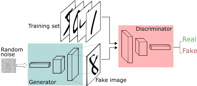
GAN composes of two types of models: Generative Model and a Discriminative Model.

Generative Models are responsible for generating different kinds of noise data whereas discriminative models are responsible to discriminate whether the given data is real or fake.

Generative models constantly trains itself to fool discriminative models by generating fake noise data and discriminative models trains itself from the training set to classify either the data is from dataset or not and not to be fooled by generative models.

Loss Function

Discriminator in GAN uses a cross entropy loss, since discriminators job is to classify; cross entropy loss is the best one out there.

This formula represents the cross entropy loss between p: the true distribution and q: the estimated distribution.

(p) and (q) are the of m dimensions where m is the number of classes.

In GAN, discriminator is a binary classifier. It needs to classify either the data is real or fake. Which means m = 2. The true distribution is one hot vector consisting of only 2 terms.

For n number of samples, we can sum over the losses.

This above shown equation is of binary cross entropy loss, where y can take two values 0 and 1.

GAN’s have a latent vector z, image G(z) is magically generated out of it. We apply the discriminator function D with real image x and the generated image G(z).

The intention of the loss function is to push the predictions of the real image towards 1 and the fake images to 0. We do so by log probability term.

Note: ~ sign means: is distributed as and Ex here means expectations: since we don’t know how samples are fed into the discriminator, we are representing them as expectations rather than the sum.

If we observe the joint loss function we are maximizing the discriminator term, which means log of D(x) should inch closer to zero, and log D(G(z)) should be closer to 1. Here generator is trying to make D(G(z)) inch closer to 1 while discriminator is trying to do the opposite.

Code for GAN

Now without any delay let’s write our GAN.

We are going to name our file art_gan.py and store it in the root directory. This file will contain all the hyperparameters and functions for our generator and discriminator.

Let’s write some code:

from keras.layers import Input, Reshape, Dropout, Dense, Flatten, BatchNormalization, Activation, ZeroPadding2D
from keras.layers.advanced_activations import LeakyReLU
from keras.layers.convolutional import UpSampling2D, Conv2D
from keras.models import Sequential, Model, load_model
from keras.optimizers import Adam
import numpy as np
from PIL import Image
import os

Here we are importing all the required libraries and helper functions for creating our GAN.

All the imports are self-explanatory. Here we are importing a bunch of keras layers for creating our models.

Now let’s define some parameters:

# Preview image Frame
PREVIEW_ROWS = 4
PREVIEW_COLS = 7
PREVIEW_MARGIN = 4
SAVE_FREQ = 100# Size vector to generate images from
NOISE_SIZE = 100# Configuration
EPOCHS = 10000 # number of iterations
BATCH_SIZE = 32GENERATE_RES = 3
IMAGE_SIZE = 128 # rows/colsIMAGE_CHANNELS = 3

Here in the first few lines, we have defined Image frame size and padding to save our generated images.

NOISE_SIZE here is a latent dimension size to generate our images.

EPOCHS is a number of iterations: it defines how many times we want to iterate over our training images and BATCH_SIZE is a number of images to feed in every iteration.

IMAGE_SIZE is our image size which we resized earlier to 128X128 and IMAGE_CHANNELS is a number of channel in our images; which is 3.

Note: Images should always be of square size

Let's load our npy data file which we’ve created earlier.

training_data = np.load(‘cubism_data.npy’)

To load the npy file we are using numpy’s load function and passing file path as a parameter.

Since we have our data file in the root directory we no additional path parameters were required. If you have stored your data somewhere else, you can use the following code to load data:training_data = np.load(os.path.join(‘dirname’, ‘filename.npy’))

That’s it for loading our training data.

Now we can create our Generator and Discriminator functions.

Let’s see that in code:

def build_discriminator(image_shape):
    model = Sequential()
    model.add(Conv2D(32, kernel_size=3, strides=2,
    input_shape=image_shape, padding=”same”))
    model.add(LeakyReLU(alpha=0.2))
    model.add(Dropout(0.25))model.add(Conv2D(64, kernel_size=3, strides=2, padding=”same”))
    model.add(ZeroPadding2D(padding=((0, 1), (0, 1))))
    model.add(BatchNormalization(momentum=0.8))
    model.add(LeakyReLU(alpha=0.2))
    model.add(Dropout(0.25))model.add(Conv2D(128, kernel_size=3, strides=2, padding=”same”))
    model.add(BatchNormalization(momentum=0.8))
    model.add(LeakyReLU(alpha=0.2))
    model.add(Dropout(0.25))model.add(Conv2D(256, kernel_size=3, strides=1, padding=”same”))
    model.add(BatchNormalization(momentum=0.8))
    model.add(LeakyReLU(alpha=0.2))model.add(Dropout(0.25))
    model.add(Conv2D(512, kernel_size=3, strides=1, padding=”same”))
    model.add(BatchNormalization(momentum=0.8))
    model.add(LeakyReLU(alpha=0.2))model.add(Dropout(0.25))
    model.add(Flatten())
    model.add(Dense(1, activation=’sigmoid’))
    input_image = Input(shape=image_shape)
    validity = model(input_image)
    return Model(input_image, validity)

breaking it down:

If you have some knowledge of keras than the code is self-explanatory.

In general, we are defining a function which takes image_shape as a parameter.

Inside that function, we are initializing a Sequential model from keras which helps us in creating linear stacks of layers.

model = Sequential()

After that, we are appending a bunch of layers in sequential model.

Our first layer is a convolutional layer of 32 shape having kernel_size of 3 and our stride value is 2 with padding same. Since it is a first layer it holds input_shape.

To understand what is going on here, you can refer to keras official documentation page.

But in simple language, here we are defining a convolutional layer which has a filter of size 3X3 and that filter strides over our image data. We have padding of same which means, no additional paddings are added. It remains the same as the original.

model.add(Conv2D(32, kernel_size=3, strides=2, input_shape=image_shape, padding=”same”))

model.add(LeakyReLU(alpha=0.2))

After that, we are adding a LeakyRelu layer which is an activation function.

Similarly in other block of layers are added in a sequential model with some dropouts and batch normalization to prevent overfitting.

The last layer of our model is a Fully connected layer with an activation function sigmoid.

Since our discriminator’s job is to classify whether the given image is fake or not, it is a binary classification task and sigmoid is an activation that squeezes every value to values between 0 and 1.

model.add(Flatten())
model.add(Dense(1, activation=’sigmoid’))

Now after initializing our discriminator model let’s create a generative model as well.

def build_generator(noise_size, channels):
    model = Sequential()
    model.add(Dense(4 * 4 * 256, activation=”relu”,       input_dim=noise_size))
    model.add(Reshape((4, 4, 256)))model.add(UpSampling2D())
    model.add(Conv2D(256, kernel_size=3, padding=”same”))
    model.add(BatchNormalization(momentum=0.8))
    model.add(Activation(“relu”))model.add(UpSampling2D())
    model.add(Conv2D(256, kernel_size=3, padding=”same”))
    model.add(BatchNormalization(momentum=0.8))
    model.add(Activation(“relu”))
    for i in range(GENERATE_RES):
         model.add(UpSampling2D())
         model.add(Conv2D(256, kernel_size=3, padding=”same”))
         model.add(BatchNormalization(momentum=0.8))
         model.add(Activation(“relu”))model.summary()
    model.add(Conv2D(channels, kernel_size=3, padding=”same”))
    model.add(Activation(“tanh”))input = Input(shape=(noise_size,))
    generated_image = model(input)
    
    return Model(input, generated_image)

Breaking it down:

Here we have defined a function that takes noise_size and channels as parameters.

Inside the function, we have again initialized a sequential model.

Since our generator model has to generate images from noise vector, our first layer is a fully connected dense layer of size 4096 (4 * 4 * 256) which takes noise_size as a parameter.

model.add(Dense(4 * 4 * 256, activation=”relu”, input_dim=noise_size))

Note: We have defined its size to be of 4096 to for resizing it in 4X4X256 shaped layer.

After that, we are using Reshape layer to reshape our fully connected layer in the shape of 4X4X256.model.add(Reshape((4, 4, 256)))

Layer blocks after this are just a Convolutional layer with batch normalizations and activation function relu.

Just to see and understand what it looks like, let’s look at the model summary:

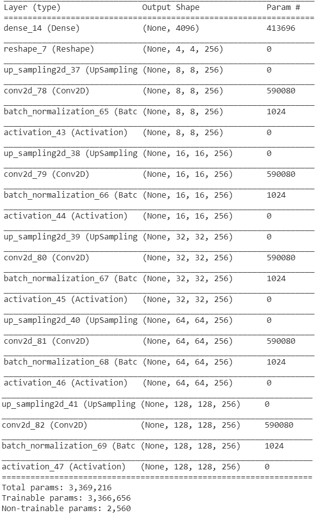
From the shape of 4X4 it is extended up to the size of 128X128 which is our training_data shape.

Our generator model takes noise as an input and outputs an image.

After initializing both the generator and discriminator model, let’s write a helper function to save the image after some iteration.

def save_images(cnt, noise):
    image_array = np.full((
        PREVIEW_MARGIN + (PREVIEW_ROWS * (IMAGE_SIZE + PREVIEW_MARGIN)),
        PREVIEW_MARGIN + (PREVIEW_COLS * (IMAGE_SIZE + PREVIEW_MARGIN)), 3),
        255, dtype=np.uint8)generated_images = generator.predict(noise)generated_images = 0.5 * generated_images + 0.5image_count = 0
    for row in range(PREVIEW_ROWS):
        for col in range(PREVIEW_COLS):
            r = row * (IMAGE_SIZE + PREVIEW_MARGIN) + PREVIEW_MARGIN
            c = col * (IMAGE_SIZE + PREVIEW_MARGIN) + PREVIEW_MARGIN
            image_array[r:r + IMAGE_SIZE, c:c +
                        IMAGE_SIZE] = generated_images[image_count] * 255
            image_count += 1output_path = 'output'
    if not os.path.exists(output_path):
        os.makedirs(output_path)filename = os.path.join(output_path, f"trained-{cnt}.png")
    im = Image.fromarray(image_array)
    im.save(filename)

Our save_images function takes to count and noise as an input.

Inside the function, it generates frames from the parameters we’ve defined above and stores our generated image array which are generated from the noise input.

After that, it saves it as an image.

Now, it’s time for us to compile the models and train them.

Let’s write a block of code for that as well:

image_shape = (IMAGE_SIZE, IMAGE_SIZE, IMAGE_CHANNELS)
optimizer = Adam(1.5e-4, 0.5)
discriminator = build_discriminator(image_shape)
discriminator.compile(loss=”binary_crossentropy”,
optimizer=optimizer, metrics=[“accuracy”])

generator = build_generator(NOISE_SIZE, IMAGE_CHANNELS)
random_input = Input(shape=(NOISE_SIZE,))
generated_image = generator(random_input)

discriminator.trainable = False

validity = discriminator(generated_image)
combined = Model(random_input, validity)
combined.compile(loss=”binary_crossentropy”,
optimizer=optimizer, metrics=[“accuracy”])

y_real = np.ones((BATCH_SIZE, 1))
y_fake = np.zeros((BATCH_SIZE, 1))

fixed_noise = np.random.normal(0, 1, (PREVIEW_ROWS * PREVIEW_COLS, NOISE_SIZE))

cnt = 1
for epoch in range(EPOCHS):
  idx = np.random.randint(0, training_data.shape[0], BATCH_SIZE)
  x_real = training_data[idx]
 
  noise= np.random.normal(0, 1, (BATCH_SIZE, NOISE_SIZE))
  x_fake = generator.predict(noise)
 
  discriminator_metric_real = discriminator.train_on_batch(x_real, y_real)
  discriminator_metric_generated = discriminator.train_on_batch(x_fake, y_fake)
 
  discriminator_metric = 0.5 * np.add(discriminator_metric_real, discriminator_metric_generated)
  generator_metric = combined.train_on_batch(noise, y_real)
  if epoch % SAVE_FREQ == 0:
     save_images(cnt, fixed_noise)
     cnt += 1
 
   print(f”{epoch} epoch, Discriminator accuracy: {100*  discriminator_metric[1]}, Generator accuracy: {100 * generator_metric[1]}”)

Breaking it down:

Here in the first few lines, we have defined our input shape: which is 128X128X3 (image_size, image_size, image_channel).

After that, we are using Adam as our optimizer.

Note: All the parameters has been sourced from the paper [1].

image_shape = (IMAGE_SIZE, IMAGE_SIZE, IMAGE_CHANNELS)
optimizer = Adam(1.5e-4, 0.5)
discriminator = build_discriminator(image_shape)
discriminator.compile(loss=”binary_crossentropy”,
optimizer=optimizer, metrics=[“accuracy”])

After initializing the optimizer, we are calling our build_discriminator function and passing the image shape then compiling it with a loss function and an optimizer.

Since it is a classification model, we are using accuracy as its performance metric.

Similarly, in the next line, we are calling our build_generator function and passing our random_input noise vector as its input.

generator = build_generator(NOISE_SIZE, IMAGE_CHANNELS)
random_input = Input(shape=(NOISE_SIZE,))
generated_image = generator(random_input)

It returns a generated image as it’s output.

Now, one important part of GAN is we should prevent our discriminator from training.

discriminator.trainable = False
validity = discriminator(generated_image)
combined = Model(random_input, validity)
combined.compile(loss=”binary_crossentropy”,
optimizer=optimizer, metrics=[“accuracy”])

Since we are only training generators here, we do not want to adjust the weights of the discriminator.

This is what really an “Adversarial” in Adversarial Network means.

If we do not set this, the generator will get its weight adjusted so it gets better at fooling the discriminator and it also adjusts the weights of the discriminator to make it better at being fooled.

We don’t want this. So, we have to train them separately and fight against each other.

We are then compiling the generative model with loss function and optimizer.

After that, we are defining two vectors as y_real and y_fake.

y_real = np.ones((BATCH_SIZE, 1))
y_fake = np.zeros((BATCH_SIZE, 1))fixed_noise = np.random.normal(0, 1, (PREVIEW_ROWS * PREVIEW_COLS, NOISE_SIZE))

These vectors are composed of random 0’s and 1’s values.

After that we are creating a fixed_noise: this will result in generating images that are saved later on which we can see it getting better on every iteration.

After that, we are going to iterate over our training data with the range of epochs we’ve defined.

cnt = 1
for epoch in range(EPOCHS):
  idx = np.random.randint(0, training_data.shape[0], BATCH_SIZE)
  x_real = training_data[idx]
 
  noise= np.random.normal(0, 1, (BATCH_SIZE, NOISE_SIZE))
  x_fake = generator.predict(noise)
 
  discriminator_metric_real = discriminator.train_on_batch(x_real, y_real)
  discriminator_metric_generated = discriminator.train_on_batch(
 x_fake, y_fake)

During the iteration process, we are taking a sample from a real image and putting that on x_real. After that, we are defining a noise vector and passing that to our generator model to generate a fake image in x_fake.

Then we are training our discriminator model in both real and fake images separately.

discriminator_metric_real = discriminator.train_on_batch(x_real, y_real)
discriminator_metric_generated = discriminator.train_on_batch(
 x_fake, y_fake)

Some research has shown that training them separately can get us some better results.

After training, we are taking the metric from both models and taking the average.

discriminator_metric = 0.5 * np.add(discriminator_metric_real, discriminator_metric_generated)

This way we get the metric for the discriminator model, now for the generator model, we are training it on our noise vector and y_real: which is a vector of 1’s.

Here we are trying to train the generator. Overtime generator will get better from these inputs and the discriminator will not be able to discriminate whether the input is fake or real.

One thing to note here, our combined model is based on the generator model linked directly to the discriminator model. Here our Input is what the generator wants as an input: which is noise and output is what the discriminator gives us.

Now in the end we have an if statement which checks for our checkpoint.

if epoch % SAVE_FREQ == 0:
 save_images(cnt, fixed_noise)
 cnt += 1
 
 print(f”{epoch} epoch, Discriminator accuracy: {100* discriminator_metric[1]}, Generator accuracy: {100 * generator_metric[1]}”)

If it reaches the checkpoint then it saves the current iteration noise and prints the current accuracy of generator and discriminator.

This is all for the coding part to create GAN, but we are not finished yet.

We have just written code for it, now we have to actually train those models and see the output how it performs.

Training GAN

Training GAN in a normal laptop is kind of impossible since it requires high computation power.

Normal laptops with normal CPUs cannot handle such huge tasks, so we are going to use Spell: Which is the fastest and most powerful end-to-end platform for Machine Learning and Deep Learning.

Why Spell?

The spell is a powerful platform for building and managing machine learning projects. The spell takes care of infrastructure, making machine learning projects easier to start, faster to get results, more organized, and safer than managing infrastructure on your own.

In every signup with Spell, you can get 10$ free credit!

In simple words, we are going to upload our data file in the spell platform and let it handle all our training task. Spell runs our task in their Powerful GPUs so that we don’t have to worry about anything. We can monitor our logs from their Web GUI and all our outputs are saved safely as well.

Training Process

There are few things to cover before running our project at Spell.

First off, we must create our account on Spell. There is good and easy documentation to get started on their official page.

After account creation, we can install Spell CLI using pip install:pip install spell

This installs all the power of spell into our laptop. We can either use the Web GUI or we can easily log in to the spell server and execute commands from our cmd or bash.

To upload our project on Spell, we are going to use command-line tools.

Let’s open the command line terminal in the root directory of our project folder and login to the server by using spell login command:spell login

After a successful login, now we can upload our training data file and run our code in the Spell server:Spell upload “filename”

After that our training_data will be uploaded to the server.

Note: Before running code in the server, code has been pushed to the github.

Now we are ready to execute our code in the Spell server.

In the command line let’s run the following command:Spell run python art_gan.py -t V100 -m uploads/art_gan/cubism_data.npy

The command above runs our code in the Spell server with the Machine type V100 which is a GPU machine. The last argument there mounts the dataset directory so that it can be accessed by our code.

Now that code is executed successfully you can see the logs on your console. If you want to monitor in GUI then you can log in to the Web GUI of Spell and see under Runs Section.

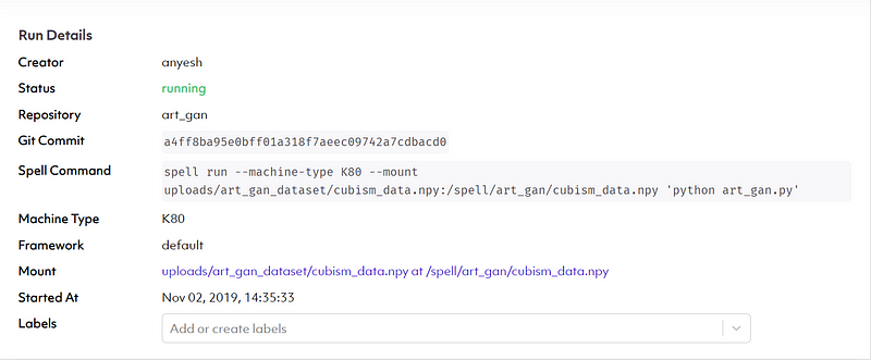
As you can see, it holds all the information about our recent run.

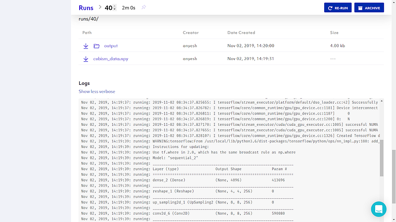
As we have written code for; in every 100th iteration our generated image is saved in the output directory and log with accuracy metric are printed.

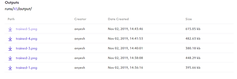
You can view them in logs section.

Awesome isn’t it? You can do your other works while it trains and saves the output for you.

Output

Now after the training completes Spell automatically saves our output in the resources/runs directory.

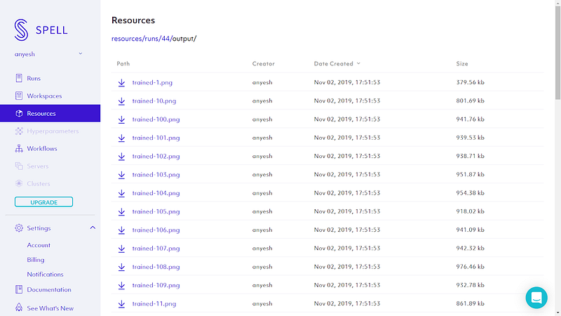
After that, we can download the outputs from the runs of Spell to our local machine by using the following command:spell cp [OPTIONS] SOURCE_PATH [LOCAL_DIR]

For this project it will be:spell cp runs/44

You just have to enter the runs/<number of your run> to download the content of that runs.

That’s it!! Now you have outputs of the GAN trained on Spell’s GPU machine in your local machine. You can now visualize how your GAN performed from that output images.

Conclusion

GANs are an exciting and rapidly changing field, delivering on the promise of generative models in their ability to generate realistic examples across a range of problem domains. It is not an easy task to understand GAN or any Machine Learning and Deep Learning field overnight. It needs patience and a lot of practice plus understanding.

In previous days it was not possible for Aspiring ML enthusiast likes us to perform repetitive practice to see what went how. But now, a platform like Spell helps us to provide a system to run and manage our projects so that we can run and test our models.

What we have created is just a simple representation of how GAN can be created and what GAN can do. There are still more advanced tweaks yet to perform.

To take it further you can tweak the parameters and see how differently it generates the images.

There are still a lot of things one can research.

For any queries and discussion, you can join the Spell community from here: https://chat.spell.ml/

Recently I built Dreamery — an AI-powered web platform to transform or generate conceptual art, studio-quality headshots cartoons and more.

References

[1] Generative Adversarial Network, Ian J. Goodfellow, Jean Pouget-Abadie, Mehdi Mirza, Bing Xu, David Warde-Farley, Sherjil Ozair, Aaron Courville, Yoshua Bengio, 2014

[2] A Gentle Introduction to Generative Adversarial Networks (GANs), Jason Brownlee, 2019 [Online] https://machinelearningmastery.com/what-are-generative-adversarial-networks-gans/

[3] A Beginner’s Guide to Generative Adversarial Networks (GANs), Chris, 2019 [Online] https://skymind.ai/wiki/generative-adversarial-network-gan